Class 1 05/06/2019

Fibonacci numbers

Fibonacci numbers (Exponential Algorithm)

0, 1, 1, 2, 3, 5, 8, 13, 21
a0, a1, a3, a3, a4, a5, a6, a7

an = an-1 + an-2
a0 = 0
a1 = 1

Code

fib1(int n) {
    if (n == 0 || n == 1) {
        return n;
    }
    return fib1(n-1) + fib1(n-2);
}

Time Complexity

Answer O(2^n)

Less intuitive, not like

1 2	for i in range(10): a[i] = a[i-1] + 2

Recursion Tree

$ T(n) = \text {runtime of fib1(n)}$

              T(n)
       /              \
    T(n-1)           T(n-2)
   /     \           /     \
T(n-2)   T(n-3)    T(n-3)   T(n-4)
            ......
T(1)    T(0)    T(1)    T(0) ...

When hit 0 or 1, the recursion ends.

            /\
           /  \
          /____\
         /     /
        /  _ /
       / _/
      /_/
left side = n
right side = n/2

T(n) = num of nodes in this recursion tree

in first half of this tree
            /\
           /  \
          /____\
num of nodes = 2^k-1 = 2 ^ (n/2) - 1

Thus we have

$ 2 ^ {n/2} <= T(n) <= 2 ^ n $

Therefore

$ 2 ^ {n/2} = (\sqrt {2}) ^ n ~= 1.4n $

Clearly, this is a bad time complexity algorithm.

                  T(n)
           /              \
        T(n-1)           T(n-2)
       /     \           /     \
    T(n-2)   T(n-3)    T(n-3)   T(n-4)

There are a lot of repetition in the process of calculation. 

e.g. T(n-2) T(n-3)

Linear algorithm

Code

fib2(int n) {
    int[] A = new int[n];
    A[0] = 0; A[1] = 1;
    for (int i = 2; i <= n; i++) {
        A[i] = A[i-1] + A[i-2];
    }
    return A[n];
}

Time Complexity

Linear time: O(n)

Constant space algorithm

Code

fib2(int n) {
    int[] A = new int[2];
    A[0] = 0; A[1] = 1;
    for (int i = 2; i <= n; i++) {
        A[i%2] = A[(i-1)%2] + A[(i-2)%2];
    }
    return A[n%2];
}

Analysis

1
2
3

i varies between 0 and 1
A[1] = A[0] + A[1]
A[0] = A[1] + A[0]

Matrix solution

Idea

$$
A = \left[
\begin{matrix}
1 & 1 \
1 & 0
\end{matrix}
\right]
$$

$$
A^2 = \left[
\begin{matrix}
1 & 1 \
1 & 0
\end{matrix}
\right] *
\left[
\begin{matrix}
1 & 1 \
1 & 0
\end{matrix}
\right] =
\left[
\begin{matrix}
2 & 1 \
1 & 1
\end{matrix}
\right]
$$

A = | 1  1 | = | a2  a1 |
    | 1  0 |   | a1  a0 |

A^2 = | 1  1 |    | 1  1 |      | 2  1 |   | a3  a2 |
      | 1  0 | *  | 1  0 |  =   | 1  1 | = | a2  a1 |

A^3 = | 2  1 |    | 1  1 |      | 3  2 |   | a4  a5 |
      | 1  1 | *  | 1  0 |  =   | 2  1 | = | a3  a2 |           

.....

 A^k = | a(k+1)  ak   |   
       | ak      ak-1 |

Time Complexity

Basic: O(n)

Optimized: O(logn)

Strategy

Since we are dealing with A^n, the optimized time complexity of pow(x, n) is O(logn)

A^n =   |A(n/2)^2         | n is even
        |A((n-1)/2)^2 * A | n is odd

A^64 = (A^32)^2 = ((A^16))^2^2 = A^(2^6)

Asymptotic Notation

Comparison of each notation

Compare Function Growth	Compare Numbers	f(n) = 5n	g(n) = n^2
O	<=	f(n) = O(g(n))
o	<	f(n) = o(g(n)
Θ	=	for f(n) = 100n	and g(n) = n + 100
Ω	>=	f(n) = Ω(g(n))
ω	>	f(n) = ω(g(n))

Mathematical Derivation

f(n) = O(g(n))

1 2	iff exists constants C and n0 s.t. when n > n0, f(n) <= C * g(n)

1
2
3

lim(n->inf) f(n)/g(n) =     0           | fn = O/o(g(n))
                            constant    | fn = O/Θ/Ω(g(n))
                            inf         | fn = Ω/ω(g(n))

Practice:

lim(n->inf) (100n)/(n+100) = 100 
fn = O/Θ/Ω(g(n))

f(n) = nlgn   g(n) = n^2
f(n) = O/o(g(n))

f(n) = 2^n   g(n) = 3^n
f(n) = O/o(g(n))
lim(n->inf) f(n)/g(n) = lim(n->inf) (2/3)^n = 0

f(n) = n+3   g(n) = 2 * sqrt(n)
f(n) = Ω/ω(g(n))


f(n) = log2(n)   g(n) = log3(n)
f(n) = Ω/O/Θ(g(n))
lim(n->inf) f(n)/g(n) = lim(n->inf) log2n/log3n = log3/log2

f(n) = (logn)^2   g(n) = log(n^2) = 2logn
f(n) = Ω/ω(g(n))

Master’s Theorem

Idea of merge sort

T(n) = 2T(n/2) + n

             T(n) n                         | n
          /          \
    T(n/2) n/2          T(n/2) n/2          | n
   /     \           /     \
T(n/4)   T(n/4)    T(n/4)   T(n/4)          | n
            ......
T(1)    T(1)    T(1)    T(1) ...            | n

Time Complexity of merge sort

T(n) = height T(level) = logn n = nlogn

Master’s Theorem

T(n) = a * T(n/b) + n^c, where a, b, c are constants

Examples:
T(n) = 2 * T(n/2) + n
T(n) = 8 * T(n/2) + n^2
T(n) = T(n/2) + 1
T(n) = T(n/3) + T(2n/3) + n  (Not master's theorem)

Now we have to compare logb(a) and c

logb(a) > c, T(n) = Θ(n^(logb(a)))
logb(a) = c, T(n) = Θ((n^c) * logn)
logb(a) < c, T(n) = Θ(n^c)

Practice

T(n) = T(n/2) + 1   T(n) = Θ(lgn)
T(n) = 8T(n/2) + n^2   T(n) = Θ(n^3)
T(n) = 7T(n/2) + n^2   T(n) = Θ(n^(log2(7)))
T(n) = 4T(n/2) + n^2   T(n) = Θ(n^2 * (logn))
T(n) = T(n/2) + n  T(n) = Θ(n)
T(n) = T(n-1) + n  (Not master's theorem)

Draw the Recursion Tree of the last one

Recursion Tree of T(n) = T(n-1) + n 

        T(n) n
        T(n-1) n-1
        T(n-2) n-2
        ...
        T(1) 1




T(n) = 1 + 2 + 3 + ... + n = n(n+1)/2
Θ(n) = n^2

Other useful Summation Formula

1 + 2 + 3 + .. + n = n(n+1)/2

q^0 + q^1 + q^2 + ... q^n = (q^(n+1) -1)/(q-1)

1 + 1/2 + 1/3 + ... + 1/n = Θ(ln(n))

Normal case

T(n) = T(n/3) + T(2n/3) + n

             T(n) n                         | n
          /          \
    T(n/3) n/3        T(2n/3)  2n/3         | n
   /     \           /     \
T(n/9)   T(2n/9)    T(2n/9)   T(4n/9)       | n
            ......
T(1)    T(1)    T(1)    T(1) ...            | n

            /\
           /  \
          /____\
          \     \
            \    \
              \   \
                \_\

left side = log3n
right side = log3/2(n)

T(n) = num of nodes in this recursion tree

n * log3(n) <= T(n) <= n * log3/2(n)

Time Complexity of Normal recursion tree

T(n) = Θ(nlgn)

Some examples

1
2
3

T(n) = T(n/4) + T(3n/4) + n             T(n) = Θ(nlgn)
T(n) = T(n/1000) + T(999n/1000) + n     T(n) = Θ(nlgn)
T(n) = T(n-1) + T(1) + n                T(n) = Θ(n^2)

Quick Sort

Partition

Given array like

|1 |9 |2 |8 |3 |8 |7 |5 |6 |


Choose a pivot, put all num < pivot in left, others in right

|    nums <=  pivot  |pivot|  nums > pivot   |

The process is partition(A[], i, j)

Code

QuickSort(int[] A, int i, int j) {
    if (i >= j) {return;}
    int pivot_pos = Partition(A, i, j);
    QuickSort(A, i, pivot_pos-1);
    QuickSort(A, pivot_pos+1, j);
}

Time Complexity

T(n) = 2T(n/2) + n = Θ(nlogn)
T(n) = T(n/3) + T(2n/3) + n = Θ(nlogn)
T(n) = T(n/1000) + T(999n/1000) + n = Θ(nlogn)

Worst Case
T(n) = T(n-1) + n = Θ(n^2)

Average T(n) = Θ(nlogn)

Worst T(n) = Θ(n^2)

Code of Partition

pivot = A[j]
| i |  ... | p | p+1 |  ...  | cur |  ...  | j |

i - p: <= pivot
p - p+1: > pivot
cur: current pointer

A[cur] > pivot
1
cur += 1
A[cur] <= pivot
1
2
3
swap(A[cur], A[p+1]);
p += 1;
cur += 1

Partition(int[] A, int i, int j) {
    int pivot = A[j];
    int p = i - 1;
    for (int cur = i; cur <= j-1; cur++) {
        if (A[cur] <= pivot) {
            swap(A[cur], A[p+1]);
            p += 1;
        }
    }
    swap(A[j], A[p+1]);
    return p+1;
}

Class 2 05/13/2019

Review

Review of quicksort

Stable Sort

| ... | 5(1) | ...  |  ...  | 5(2) |  ...  |

After sort

| ... | 5(1)| 5(2) |  ...  |

If two 5 are still in their relative positions, then this is a stable sort.

Runtime of Quick Sort

Runtime:

Average: $O(nlogn)$
Worst: $O(n^2)$

The worst case is $T(n) = T(n-1) + n$

Pivot Selection

Median of Three

1	\| i \| ... \| (i+j)/2 \| ... \| j \|

Heap Sort

Types of Heap

Max Heap
Min Heap

Operations (of Heap)

Insert(E) $O(logn)$
getMax() $O(1)$
deleteMax() $O(logn)$

Operations (of Sorted Array)

Insert(E) $O(n)$
getMax() $O(1)$
deleteMax() $O(1)$

Comparison of array and heap

The worst time of heap operation is logn.

However, A sorted array takes On time to insert, which is the bottleneck of the overall time complexity.

Logical View and Physical View

Logical View


          7(1)
         /    \
      3(2)      6(3)
     /   \       /
   1(4)  2(5)  5(6)

Almost-Full Binary Tree
Parent must be >= both children

Physical View

1
2
3


               1   2   3   4   5   6
Array        | 7 | 3 | 6 | 1 | 2 | 5 |

helper functions of heap

i is the index

parent(i) = i / 2
leftChild(i) = i 2
rightChild = i 2+1

getMax() O(1)

getMax() - return A[1]

insert() O(logn)

Case 1

           7(1)
         /      \
      3(2)      6(3)
     /   \       / \
   1(4)  2(5)  5(6) 3(7)

No need to adjust

Case 2

           7(1)
         /      \
      3(2)      6(3)
     /   \       / \
   1(4)  2(5)  5(6) 8(7)

Swap 8 with 6

           7(1)
         /      \
      3(2)      8(3)
     /   \       / \
   1(4)  2(5)  5(6) 6(7)

Swap 7 with 8

           8(1)
         /      \
      3(2)      7(3)
     /   \       / \
   1(4)  2(5)  5(6) 6(7)  

Complete inserting.

                        1   2   3   4   5   6   7
Array(after insert)   | 8 | 3 | 7 | 1 | 2 | 5 | 6|

Code of insert()

void insert(int e) {
    // increase the size n of the heap
    n += 1;
    // insert the item to heap A
    A[n] = e;
    // Adjust from index i=n
    int i = n;
    // if cur node has a parent and the parent is smaller
    while (parent(i) > 0 && A[parent(i)] < A[i]) {
        swap(A[parent(i)], A[i]);
        i = parent(i);
    }
}

deleteMax()

           8(1)
         /      \
      3(2)      7(3)
     /   \       / \
   1(4)  2(5)  5(6) 6(7)  

Swap 6 with 8, and delete 8

           6(1)
         /      \
      3(2)      7(3)
     /   \       / 
   1(4)  2(5)  5(6) 

                      1   2   3   4   5   6  
Array(after swap)   | 6 | 3 | 7 | 1 | 2 | 5 | 

Swap 6 with 7

           7(1)
         /      \
      3(2)      6(3)
     /   \       / 
   1(4)  2(5)  5(6) 

                      1   2   3   4   5   6  
Array(after swap)   | 7 | 3 | 6 | 1 | 2 | 5 | 

Heap is balanced. 
deleteMax() completed.

heapify()

           6(1)
         /      \
      3(2)      7(3)
     /   \       / 
   1(4)  2(5)  5(6)  

The subTree of root 3 is a MaxHeap
The subTree of root 7 is a MaxHeap
However, the tree of root 6 is not a MaxHeap.
Now we need the heapify().

Code of heapify()

void heapify(int[] A, i) {
    int largest = i;
    // Find the largest of cur root(i) and its children
    // if left child exists and left child is bigger than cur root
    if (leftChild(i) <= n && A[leftChild(i)] > A[largest]) {
        largest = leftChild(i);
    }
    // if left child exists and left child is bigger than cur root
    if (rightChild(i) <= n && A[rightChild(i)] > A[largest]) {
        largest = rightChild(i);
    }

    // check largest
    if (largest == i) return;

    // let the cur largest node be the root
    swap(A[i], A[largest]);
    // continue heapifying down the swapped node recursively
    heapify(A, largest);
}

Code of deleteMax()

void deleteMax() {
    // swap the cur root with the last node
    swap(A[1], A[n]);
    // delete the last node
    n -= 1;
    // heapify the whole heap
    heapify(A, 1);
}

Heap Sort

Max Heap

          1   2   3   4   5   6  
Array   | 7 | 3 | 6 | 1 | 2 | 5 | 

Pretend we are deleting the max val.(deleteMax())

                         1   2   3   4   5 || 6  
Array(after deleted)   | 5 | 3 | 6 | 1 | 2 || 7(max) |
Now we get the biggest node in the tail of the array.
continue sort the rest.

Code of Heap Sort

void heapSort(int[] A) {
    for(int i = n; i >= 1; i--) {
        deleteHeap(A, 1, i);
    }
}

makeHeap()

Solution 1 insert n times O(nlogn)

Solution 2

           6(1)
         /      \
      3(2)      7(3)
     /   \       / 
   1(4)  2(5)  5(6)  

n = 3 is the last non-trivil node
we heapify the 7, 3, 6 nodes, where we ensure that all children are valid heap.

Code of makeHeap()

// On time 
// n/2 means the last non-trivil node in the heap
for (int i = n/2; i >=1; i--) {
    heapify(A, i);
}

Example of heap sort

First, make this into a heap.

           9(1)
         /      \
      2(2)      6(3)
     /   \       / 
   1(4)  4(5)  3(6)  

          1   2   3   4   5   6  
Array   | 9 | 2 | 6 | 1 | 4 | 3 |    

call makeHeap() on 6

call makeHeap() on 2

           9(1)
         /      \
      4(2)      6(3)
     /   \       / 
   1(4)  2(5)  3(6)  

          1   2   3   4   5   6  
Array   | 9 | 4 | 6 | 1 | 2 | 3 |  

call deleteHeap() on 9

           3(1)
         /      \
      4(2)      6(3)
     /   \       
   1(4)  2(5)  

          1   2   3   4   5    6  
Array   | 3 | 4 | 6 | 1 | 2 || 9 |

call heapify() on 3

           6(1)
         /      \
      4(2)      3(3)
     /   \       
   1(4)  2(5)  

          1   2   3   4   5    6  
Array   | 6 | 4 | 3 | 1 | 2 || 9 |

call deleteHeap() on 6

           2(1)
         /      \
      4(2)      3(3)
     /       
   1(4)  

          1   2   3   4    5   6  
Array   | 2 | 4 | 3 | 1 || 6 | 9 |

call heapify() on 2

           4(1)
         /      \
      2(2)      3(3)
     /         
   1(4)   

          1   2   3   4    5   6  
Array   | 4 | 2 | 3 | 1 || 6 | 9 |

call deleteHeap() on 4

           1(1)
         /      \
      2(2)      3(3)
     /          
   4(4)   

          1   2   3    4   5   6  
Array   | 1 | 2 | 3 || 4 | 6 | 9 |
...
The array is sorted.

Sorting Algorithms

Types of sorting algorithms

Algorithm	Time Complexity	Notes
Quick Sort	$O(nlogn)$
Merge Sort	$O(nlogn)$
Heap Sort	$O(nlogn)$
Bubble Sort	$O(n^2)$
Insertion SOrt	$O(n^2)$
Selection SOrt	$O(n^2)$
Counting SOrt	$O(n)$	Non-comparison based
Radix SOrt	$O(n)$	Non-comparison based

Theorem of comparison based sorting algorithm

Comparison based sorting algorithm always run in $Ω(nlogn)$.

Counting Sort

Assume we have array A
The input nums should satisfy 0 <= A[i] <= k

input   A    | 2 | 1 | 3 | 5 | 4 | 2 | 1 | 0 | 3 |

               0   1   2   3   4   5
bucket  B    | 1 | 2 | 2 | 2 | 1 | 1 |

               0   1   2   3   4   5
bucket  B'   | 1 | 3 | 5 | 7 | 8 | 9 |

output  C    | 0 | 1 | 1 | 2 | 2 | 3 | 3 | 4 | 5 |

Code of Counting Sort

//Step of counting sort
// fill the num in the buckets
for (int i = 0; i < n; i++) {
    B[A[i]] += 1
}

// indicates where the curr digit ends in the ouput array
for (int i = 1; i <= k; i++) {
    B[i] += B[i-1];
}

// fill the digit into the array
for (int i = n-1; i >= 0; i--) {
    C[B[A[i]]] = A[i];
    B[A[i]] -= 1;
}

return C;

problems of Counting Sort

Q: Why 0-based?
A: To represent the case where the input has 0.

Q: what happened if we have negative input?
A: Map the input to the form we want. e.g. [-10, 10] -> [0, 20]

Q: Is this algorithm stable?
A: In this case, yes.

Analysis of Counting Sort

Run time: $O(n+k)$
Space: $O(k)$

Radix Sort

Introduction

Also known as digit sort.

Only for positive base 10 integers.

Example

Use the counting sort to sort the colomn

100      100     100       4
 23       41       4      13
123      512     512      23  
512       23     013      41
  4  =>  123 =>   23  => 100
 13       13     123     123
 41        4      41     512
999      999     999     999

Analysis

d is the number of digits, k is the range of the inputs(e.g. 32 bit integer)
Run time: $O((n+k)d)$
Space:

e.g.

32-bit int
| 8-bit | 8-bit | 8-bit | 8-bit |  
d = 4 times of counting sort
k = 2^8 = 256

Class 3 05/20/2019

Questions about Order Statistics

Given a collection of integers, get the min/max value, median, 25% element, rth smallest element, etc.

Question: How do we find the rth smallest element?

Solution1 Sort the array

sort array
return A[k]

The run time should be O(nlgn)

Solution2 Based Partition

Idea

Definition 2

| 1 | ... | start | ... | end | ... | 10 |

A   | 1 | 2 | 3 | 6 | 7 | 5 | 4 |

pos = partition(A, 1, 7, 5)
pos = 3

if we get the 3 as the pivot position, which means we still have to find 2 more elements

we continue searching on kth(A, 4, 7, 2)

Code

// definition 1
int findKth(int[] A, int k) {
    int pos = partition(A, 1, n);
    if (pos == k) return A[k];
    if (pos > k) return findKth(A, 1, pos);
    if (pos < k) return findKth(A, pos+1, n);
}

// definition 2
// global index
// rank of number with A[begin...end]
int findKth(int[]A, int begin, int end, int k) {
    
}

Analysis

$ T(n) = T(n/2) + n = O(n)$

Example 
T(n) = T(2n/3) + n = O(n)
T(n) = T(99n/100) + n = O(n)
T(n) = T(n-1) + n = O(n^2)

Find Top K

Solution 1 Sort the array

Sort the array
return A[1:k]

Time: $ O(nlogn) $

Solution 2 findKth algorithm

partition
return A[1:k]

Time: $ O(n) $

Solution 3 Min Heap

make a min heap
delete k times

Time: $O(n + klogn)$ (depends on which one’s bigger)

Solution 4 Max Heap

m make a max heap A[1:k]

for (i = k+1, ... , n)
    if(A[i] < getMax()) {
        deleteMax();
        insert(A[i]);
    }

Time: $ O(k + (n-k)*logk)$
When n is large, $ O(nlogk) $
When k is large, $ O(k) $

Big Integer Multiplication

for integers of 32-bit(unsigned), we have a range of $ (0, 2^{32}-1) $, which are 10 digits

for integers of 64-bit(unsigned), we have a range of $ (0, 2^{64}-1) $, which are 10 digits

RSA

An encryption algorithm using large integer multiplication.

Idea

Input: 2 integers of n-bits
Example:

1
2
3

    1110 = 14
*   0101 =  5
 1000110 = 70

Time : $ O(n^2) $

Divide and Conquer

a can be split to a1 | a2

for example,
a = 1110 = $ 11 * 2^2 + 10 $ (Shift left by 2 bit)

Therefore,
$ a = a_12^{n/2} + a_2 $
$ b = b_12^{n/2} + b_2 $
$ a b = a_1b_12^{n} + (a_1b_2+a_2b_1)2^{n/2} + a_2b_2 $

We divide the 1 problem to 4 child problem.

T(n) = 4T(n/2) + n(sum 2 n-bit integers) = O(n^2)

Improve the running time

$ p_1 = a_1b_1$
$ p_2 = a_2b_2$
$ p_3 = (a_1+a_2)(b_1+b_2)$
$ a b = p_12^{n} + (p_3-p_1-p_2)2^{n/2} + p_2 $

We can save the Time to

T(n) = 3T(n/2) + n
$ T(n) = O(n^{log_2{3}}) $

Extra cases

What if 2 integers are not with the same digits?
Pad the 0’s to the nearest exponential of 2.

1
2
3

For example
110 -> 0110
10010 -> 00010010

Square Matrix Multiplication

Idea

input: 2 n*n matrices

$
X = \left[
\begin{matrix}
A & B \
C & D
\end{matrix}
\right]_{n*n}
$

$Y = \left[
\begin{matrix}
E & F \
G & H
\end{matrix}
\right]_{n*n}
$

$ X*Y = O(n^3) $

Here we use the block of matrix to Divide & Conquer

$
X = \left[
\begin{matrix}
1 & 1 \
1 & 0
\end{matrix}
\right]_{n*n} = \left[
\begin{matrix}
A & B \
C & D
\end{matrix}
\right]
$

$Y = \left[
\begin{matrix}
1 & 1 \
1 & 0
\end{matrix}
\right]_{n*n} = \left[
\begin{matrix}
E & F \
G & H
\end{matrix}
\right]
$

$ XY = \left[
\begin{matrix}
{AE+BG} & {AF+BH} \
{CE+DG} & {CF+DH}
\end{matrix}
\right]_{nn}
$

Therefore, $ T(n) = 8T(\frac{n}{2}) + n^2 = O(n^3)$

Optimization

$ XY = \left[
\begin{matrix}
{AE+BG} & {AF+BH} \
{CE+DG} & {CF+DH}
\end{matrix}
\right]_{nn} = \left[
\begin{matrix}
{Q} & {R} \
{S} & {T}
\end{matrix}
\right]
$

$Assume:$
$P_1 = A(F-H)$
$P_2 = H(A+B)$
$P_3 = E(C+D)$
$P_4 = D(G-E)$
$P_5 = (A+D)(E+H)$
$P_6 = (B-D)(G+H)$
$P_7 = (A-C)(E+F)$
$Q = P_4 + P_5 - P_2 + P_6$
$R = P_1 + P_2$
$S = P_3 + P_4$
$T = P_1 + P_5 - P_3 - P_7$

$ X*Y = \left[
\begin{matrix}
{AE+BG} & {AF+BH} \
{CE+DG} & {CF+DH}
\end{matrix}
\right] = \left[
\begin{matrix}
{P_4 + P_5 - P_2 + P_6} & {P_1 + P_2} \
{P_3 + P_4} & {P_1 + P_5 - P_3 - P_7}
\end{matrix}
\right]
$

Therefore, $ T(n) = 7T(\frac{n}{2}) + n^2 = O(n^3)$, Successfully optimized.

Counting Inversions

Idea

Inversion: if i < j && A[i] > A[j], then (i, j) is an inversion.

If my favorite list is [1, 2, 3], num of inversion is 0
If list is [2, 1, 3], num of inversion is 1
If list is [2, 3, 1], num of inversion is 2
If list is [3, 2, 1], num of inversion is 3, we have a completely different taste

Max num of inversions of a n list is $ C^{2}_{n} = O(n^2) $

Code

// Brute force
int count = 0;
for (int i = 0; i <=n; i++) {
    for(int j = i+1; j <=n; j++) {
        if (A[i] > A[j]) {
            count++;
        }
    }
}

Better Implementation


        1         n/2 n/2+1       n
A       |      x     |       y    |

num of cross inversions + x + y


        begin        mid mid+1      end
A       |     1  3  5   |  0  2  6   |
              p            q

given A[p] = 1, A[q] = 0, A[p] > A[q], we have inv += 3, q++
A[p] < A[q], p++
A[q] < A[p], inv += 2, q++
A[p] < A[q], p++
A[p] < A[q], p++, end

Code

int CountInv(int[] A, int begin, int end) {
    if (begin >= end) return 0;
    int mid = (mid + end) / 2;
    int x = CountInv(A, begin, mid);
    int y = CountInv(A, mid+1, end);
    int z = CrossInv(A, begin, mid, end);
    return x + y + z;
}

// o nlogn time
int CrossInv(int[] A, int begin, int mid, int end) {
    sort(A, begin, mid);
    sort(A, mid+1, end);
    int p = begin, q = mid + 1, count = 0;
    while (p <= mid && q <= end) {
        if (A[p] < A[q]) p++;
        else {
          count += mid - p+1;
          q++;
        }
    }
    return count;
}

Analysis

$ T(n) = 2T(\frac{n}{2}) + nlogn = O(nlognlogn)$

Optimization

int CountInv(int[] A, int begin, int end) {
    if (begin >= end) return 0;
    int mid = (mid + end) / 2;
    int x = CountInv(A, begin, mid); // sort the left
    int y = CountInv(A, mid+1, end); // sort the right
    int z = CrossInv(A, begin, mid, end); // count the cross
    //merge left and right 
    merge(A, begin, mid, end);
    return x + y + z;
}

// on time
int CrossInv(int[] A, int begin, int mid, int end) {
    int p = begin, q = mid + 1, count = 0;
    while (p <= mid && q <= end) {
        if (A[p] < A[q]) p++;
        else {
          count += mid - p+1;
          q++;
        }
    }
    return count;
}

$ T(n) = 2T(\frac{n}{2}) + n = O(nlogn)$

Example

        | 7 | 2 | 3 | 4 | 1 | 6 | 5 | 8 |
        | 2 | 3 | 4 | 7 | 1 | 6 | 5 | 8 |
                    /    \ 
           3                    
  | 2 | 7 | 3 | 4 |         | 1 | 6 | 5 | 8 |

    /       \                   /       \
   1         0                 
| 7 | 2 |  | 3 | 4 |        | 1 | 6 |   | 5 | 8 |

Class 4 06/03/2019

Binary Search Tree and Hashtable

Difference between two data structures

Hashing	BST
O(1)	h	insert(key,value)
O(1)	h	lookup(key)
O(1)	h	delete(key)
amartized running time	O(logn) basically
	support traversing by ordered keys

Binary Search Tree

Definition

class Node {
    int key;
    Node left;
    Node right;
}

     5
   /   \
  3     8
   \
    4
This is a BST

     5
   /   \
  3     8
   \
    6
This is not a BST

Left subtree is BST
Right subtree is BST
root.key > all keys in left subtree
and root.key < all keys in right subtree

Tree Traversals

Level-order
Pre-order
Post-order
In-order

Level-order Traversal

void LevelOrder(Node root) {
    Queue<Node> q = new LinkedList<>();
    q.offer(root);
    while (!q.isEmpty()) {
        Node cur = q.poll();
        // processing on cur; print cur.key;
        if (cur.left != null) q.offer(cur.left);
        if (cur.right != null) q.offer(cur.right);
    }
}

Right Side View Question

     5
   /   \
  3     8
   \
    4
we get the right side view as [5, 8, 4]

// we can just modify the original code by
cur, curLevel = q.dequeue();
res[cur_level] = cur.key


class Solution {
    // level order traversal 
    // on time on space
    public List<Integer> rightSideView(TreeNode root) {
        List<Integer> res = new LinkedList<>();
        if (root == null) return res;
        LinkedList<TreeNode> queue = new LinkedList<>();
        queue.offerLast(root);
        int size = 1;
        while (!queue.isEmpty()) {
            int temp=0;
            for (int i = 0; i < size; i++) {
                TreeNode cur = queue.pollFirst();
                if (cur.left != null) queue.offerLast(cur.left);
                if (cur.right != null) queue.offerLast(cur.right);
                temp = cur.val;
            }
            res.add(temp);
            size = queue.size();
        }
        return res;
    }
}

Pre-order Traversal

void PreOrder(Node cur) {
    if (cur == null) return;
    Process(cur);
    PreOrder(cur.left);
    PreOrder(cur.right);
}

In-order Traversal

     5
   /   \
  3     8
   \
    4
we get the inorder node list as [3, 4, 5, 8], which is  sorted.

Represent duplicate keys in BST

Requirement

Has to support root >= all left and root < all right.

MultiSet
MultiMap

Implementation

Lookup

boolean Lookup(Node cur, int key) {
    if (cur == null) return false;
    if (cur.key == key) return true;
    if (cur.key < key) return Lookup(cur.right, key);
    return Lookup(cur.left, key);
}

Insert

Node insert(Node cur, int key, String val) {
    if (cur == null) return new Node(key, val);
    if (key == cur.key) cur.val = val;
    else if (key < cur.key) {
        cur.left = insert(cur.left, key, val);
    } else {
        cur.right = insert(cur.right, key, val);
    }
    return cur;
}

Delete

          5
        /   \
       3     6
     /  \
    2    4

Delete 5(2 children)

          4
        /   \
       3     6
     /  
    2

Case 1: No children
update parent’s reference

Case 2: Single child
Parent pointing to child

Case 2: two children

find predecessor p
swap
delete recursively

# Definition for a binary tree node.
# class TreeNode:
#     def __init__(self, x):
#         self.val = x
#         self.left = None
#         self.right = None

class Solution:
    # O logn time O logn space
    # Recursion
    # recursively find the root to delete
    # 3 edge cases
    # if no children, then simply return None
    # if 1 left child, then find the predecessor, swap, and delete the predecessor
    # if 1 right child, then find the successor, swap, and delete the successor
    # in common case, a node has both children, in this case we can find the predecessor as newNode or successor as new Node
    def deleteNode(self, root: TreeNode, key: int) -> TreeNode:
        if not root:
            return None
        if root.val > key:
            root.left = self.deleteNode(root.left, key)
        elif root.val < key:
            root.right = self.deleteNode(root.right, key)
        else:
            if not root.left and not root.right:
                root = None
            elif root.left:
                root.val = self.getPrev(root)
                root.left = self.deleteNode(root.left, root.val)
            else:
                root.val = self.getNext(root)
                root.right = self.deleteNode(root.right, root.val)
        return root
    def getPrev(self, root):
        temp = root.left
        while temp.right:
            temp = temp.right
        return temp.val
    def getNext(self, root):
        temp = root.right
        while temp.left:
            temp = temp.left
        return temp.val

Class 5 06/10/2019

Recap of BST

Predecessor and Successor

Logical view

          5
        /   \
       3     8
     /  \   /  \ 
    2    4 6    10
   /        \
  1          7
pre(8) = 7
pre(6) = 5

Predecessor

case1: rightmost node of the left subtree
case2: find smaller node on the ancestor path

Re-Definition of node

class Node {
    int key;
    Node left;
    Node right;
    Node parent;
}

Find Kth key in BST

Idea of In-order traversal

We can find the kth key by stopping at kth step during in-order traversal.

Our goal is to control the time in O(h).

Re-definition of Node

class Node {
    int key;
    Node left;
    Node right;
    Node parent;
}

Logical View

      5(5)
    /      \
   3(3)     10(1)
 /    \   
2(1)   4(1)

Code

int kth(Node root, int k) {
    rank = root.left.size + 1;
    if (rank == k) return root;
    if (rank < k) return kth(root.right, k - rank);
    return kth(root.left, k);
}

Example

          5(5)
        /      \
       3(3)     10(1)
     /    \   
    2(1)   4(1)

to find kth(4), rank = 4 = k, we just return 5

to find kth(3), rank = 2 < k, we call the func on 4(1), rank = 1 = k, return 4

Hashing/ HashTable

Pre-hash and Hash

Difference

Pre-Hash	Hash
int/float/string/user-define -> int	arbitrary large int -> reasonable int
Can only return small integers

Example

HashTable<String , T> means we have String as key, T as value.

class Pair {
    int x;
    int y;
}

HashTable<Pair, T> means we represent a coordinate as key.

In java, we overwrite the HashCode() as the pre-hash function.

For a String , a practical pre-hash function would be calculating the ascii code.

ASCII is a 8 bit representation of a char data type.

e.g.

For “hello” and “hell”, we have

1 2	Hashcode("hello") = 'h' * 41^3 + 'e' * 41^2 + 'l' * 41^1 + 'l'

p.s. the hashcode of single letter depends on the encoding way. If simple english, we just use its ascii. If unicode, we use another way.

e.g. To represent Pair, we can use x^y as its hash function.

SubSet : We can split the string and calculate each part of it, while we have a bigger chance to collision and worse time consumption.
Caching : For extra long String, we can only call the hash function once, and store the pre-hash value in the memory.

HashTable

Idea

key = Integer[in large space]
Suppose key ranges from (0, m-1), then we have to map the integer from 0 to m-1
insert(key)
hash: int -> int [0, m)

How do we choose m?

m changes dynamically

Load Factor $ \alpha = n/m $
n = number of k-v pairs
m = size of current hashtable
Here, we increase m exponentially.
e.g. m = 1024, next m would be 2048

Question: Why don’t we increase m by 100 each time?
Answer: Suppose we have $ \alpha = 1$, then every time we hit the bottle neck, we have to find a continuous memory to store all the stuff, which is a expensive On operation.

Question: what happens if we do insert n times with m increasing by 100?
Answer:

C, C, C, ..., C, 100C
C, C, ..., 200C
C, C, ..., 300C
C, C, ..., n/100C

Overall: 100 + 200 + 300 + .. n/100 ~= O(n^2) time, which is super expensive. 

C, C, C, ..., C, n/lognC
C, C, ..., n/8C
C, C, ..., n/4C
C, C, ..., n/2C

Overall: n/logn + n/8 + n/4 + .. n/2 ~= O(n) time, which is much better.

Question: what happens if we have to adjust the size?
Answer: Suppose $ \alpha < 0.2$, we would like to shrink the size by half. If $ \alpha > 0.8$, we would like to double the size. The threshold shold be decided wisely.

what should be the hash function?

hash function: (large space)int -> int [0, m)

Division Method

$ H(x) = x \% m $

If m is a power of 2, then this function is bad. e.g. If m = 1024, if pre-hash only consists of even numbers, then half of the space is wasted. We should pick prime number as m. (disadvantage)

Multiplication Method

$ H(x) = a * x \% 2^{32} >> (32 - r) $
$ m = 2^r $
a is constant chosen randomly.

Explanation: Since m = 2^r, we only need r bit to represent the hashcode. Suppose x is 32 bit, and a is 32 bit, then a*x is 64 bit. Then we mod it by 2^32, where we throw away half of the number. Next we right shift till we get only r digits, so that the hashtable con contain the num.

1
2
3

x = | 1 | 1 | 0 | ... | 1 | 0 | 1| (32)
a = | 0 | 0 | 1 | ... | 1 | 0 | 1| (32)
a is random and every 1 means we duplicate a x and left shift by x k digits. In this way the middle part is more random than right part, because e use more information of thee original x in the middle(than the edge).

Collision

Birthday Paradox

Suppose we randomly select x people, what’s the probability that two people have same birthday?

To get a 50% of prob, we should select 23 people.

This example showws the impact of collision.

There are 2 ways to deal with collision, Chaining, Probing.

Chaining

$ h(x_{1}) = k $
$ h(x_{2}) = k $
Then we have key k -> $x_1$ => $x_2$

run time O(1 + $ \alpha $)
$ \alpha $ is load factor n/m
worst case insert: len n/m logn

Probing

Here we are talking about Linear Probing.

$ h(x_{1}) = k $
$ h(x_{2}) = k $
Then we have key k ($x_1$) -> n slots taken -> (k+n) $x_2$

Delete: When wew delete an element, all the following elements have to be re-hashed.

Suppose $ \alpha = n/m = 0.1$
90 % of time is empty
Therefore we need $1 / (1-\alpha)$ space to get a slot.

time complexity: O n

Class 6 06/17/2019

Dynamic Programming

Steps of DP problem

Situations of DP
- Optimization : max/min problem
- Counting: binomial
- Feasibility: if the target is possible to get
Design recursion
Naive recursive implementation yields bad running time(Usually exponential)
- e.g. Recompute the same thing. Fibonacci.
Caching
- bottom -> up( small -> large)
- top -> down with memoization

Longest Common Subsequences

Description

input: A[1 ... n]
       B[1 ... n] 
e.g.
A = [1, 5, 2, 3, 4]
sub can be [1]  [1, 3]  [1, 2, 4]
not [3, 2, 4]

Solution

define f(i, j) = length of the LCS given A[1 ... i] & B[1 ... j]

A | 1 | ... | i |
B | 1 | ... | j |

case 1: A[i] = B[j]
f(i, j) = f(i-1, j-1) + 1

case 2: A[i] != B[j]
f(i, j) = max(f(i-1, j), f(i, j-1))

base case: f(0, j) = f(i, 0) = 0

Pseudocode

// O 2^n time O m+n space
int LCS_slow(int[] A, int[] B, int i, int j) {
    if (i == 0 || j == 0) return 0;
    if (A[i] == B[j]) return 1 + LCS_slow(A, B, i-1, j-1);
    return Math.max(LCS_slow(A, B, i, j-1), LCS_slow(A, B, i-1, j));
}

// 2-d array dp(bottom up)
// O mn time O mn space
int LCS(int[] A, int[] B, int i, int j) {
    for (int i = 0 ... n) dp[i, 0] = 0;
    for (int j = 0 ... m) dp[0, j] = 0;
    for (int i = 1 ... n) {
        for (int j = 1 ... m) {
            if (A[i] == B[j]) dp[i][j] = dp[i-1][j-1] + 1;
            else dp[i][j] = max(dp[i-1, j], dp[i, j-1]);
        }
    }
    return dp[n, m]
}

// optimized recursive solution (top down)
int LCS(int[] A, int[] B, int i, int j, int[][] dp) {
    if (i == 0 || j == 0) return 0;
    if (dp[i][j] != -1) return dp[i][j];
    if (A[i] == B[j]) {
        dp[i][j] = LCS(A, B, i-1, j-1, dp) + 1;
    } else {
        dp[i][j] = Math.max(LCS(A, B, i-1, j, dp), LCS(A, B, i, j-1, dp));    }

    return dp[i][j];
}

// get the result set out of 2-d ap array
// O m+n time
int constructSolution(int[] A, int[] B, int[][] dp) {
    List<Integer> l = new ArrayList<>();
    int i = A.length;
    int j = B.length;
    while (i > 0 && j > 0) {
        if (A[i] == B[j]) {
            l.add(A[i]);
            i--;
            j--;
        } else if (dp[i-1][j] < dp[i][j-1]) {
            j--;
        } else i--;
    }
    return l.reverse();
}

// optimized space solution
// O min(m, n) space O mn time
// dp row = 2, col = n
int LCS(int[] A, int[] B, int i, int j) {
    for (int i = 1 ... n) {
        for (int j = 1 ... m) {
            if (A[i] == B[j]) dp[i%2][j] = dp[(i-1)%2][j-1] + 1;
            else dp[i%2][j] = max(dp[(i-1)%2, j], dp[i%2, j-1]);
        }
    }
    return dp[n, m]
}

Code(Bottom Up)

def func(A, B):
    m = len(A)
    n = len(B)
    dp = [[0 for _ in range(n+1)] for _ in range(m+1)]
    for i in range(1, m+1):
        for j in range(1, n+1):
            if A[i-1] == B[j-1]:
                dp[i][j] = dp[i-1][j-1]+1
            else:
                dp[i][j] = max(dp[i][j-1], dp[i-1][j])
    return dp[m][n]

int lcs(int[] A, int[] B) {
    int m = A.length;
    int n = B.length;
    int[][] dp = new int[m+1][n+1];
    for (int i = 1; i < m+1; i++) {
        for (int j = 1; j < n+1; j++) {
            if (A[i-1] == B[j-1]) dp[i][j] = dp[i-1][j-1] + 1;
            else dp[i][j] = Math.max(dp[i-1][j], dp[i][j-1]);
        }
    }
    return dp[m][n];
}

List<Integer> constructSolution(int[] A, int[] B, int[][] dp) {
    List<Integer> l = new ArrayList<>();
    int i = A.length;
    int j = B.length;
    while (i > 0 && j > 0) {
      if (A[i] == B[j]) {
        l.add(A[i]);
        i--;
        j--;
      } else if (dp[i-1][j] < dp[i][j-1]) {
        j--;
      } else i--;
    }
    Collections.reverse(l)
    return l;
  }

0-1 Knapsack Problem

Description

Assume we have n items
value = [...]
weight = [...]
capcity = C
We need to get the max value.
f(i, j) = item[0-i], capacity j
f(i, j) = max(v[i] + f(i-1, j-weight[i]), f(i-1, j))

base case
f(0, j) = f(i, 0) = 0

Pseudocode

// O N*C time O n*c space -> O C space(optimized)
int knapsack(int[] values, int[] weights, int C) {
    for (int i = 0; i < values.length; i++) {
        for (int j = 0; j <= C; j++) {
            if (weights[i] <= j) {
                dp[i][j] = Math.max(dp[i-1][j], values[i] + dp[i-1][j-weights[i]];)
            } else {
                dp[i][j] = dp[i-1][j];
            }
        }
    }
    return dp[n][j];
}

Class 7 06/24/2019

Unbounded Knapsack

Description

Input: n types of items, for each type there are inf copies. For each item of type i, we have values[i] and weights[i]. We also have capacity of knapsack.

Naive approach

f(i) maximum value we can get
f(i) = max value given capacity i

a1 = V[1] + f(i-w[1])
a2 = V[2] + f(i-w[2])
...
a3 = V[3] + f(i-w[3])
f(i) = max(v[1], v[2], ... v[n])

base case:
f(0) = 0
T(n) -> n sub problems each time -> O(n^C)

Pseudocode

// O Cn time O C space
int knapsack(int[] v, int[] w, int C) {
    int[] dp = new int[C+1];
    for (int i = 1; i <= C; i++) {
        for (int j = 0; j < v.length; j++) {
            if (w[j] <= i) dp[i] = Math.max(dp[i], v[j] + dp[i-w[j]]);
        }
    }
    return dp[C];
}

Coin Change

Description

1
2
3

Assume we have coins like 
d1 = 1, d2 = 5, d3 = 10, d4 = 25
If we have to get total = 3.37$, what's the minimum number of coins do we have to pick?

Naive approach

f(i) = min(
    f(i - d[k]) + 1,
    f(i - d[k-1]) + 1,
    ...
    f(i - d[1]) + 1,
)

PseudoCode

int coinChange(int[] d, int n) {
    int[] dp = new int[n+1];
    for (int i = 1; i <= n; i++) {
        dp[i] = i;
        for (int j = 0; j < d.length; j++)  {
            if (d[i] <= i) {
            dp[i] = Math.min(dp[i], dp[i-d[k]] + 1);
            }
        }
    }
    return dp[n];
}

Knapsack with multiple constraints

Description

Now the items have a volume constraint
n items  v[i], w[i], u[i]
W - weight capacity
U - volume capacity
Only 1 copy of each item
What's the maximum value we can get?

Recursion

i = # of items of first i items
j = remaining weight capacity
k remaining volume capacity
f(i, j, k) = max value with constraints
f(i, j, k) = max(
    f(i-1, j, k), 
    f(i-1, j-w[i], k-u[i]) + v[i]
)

base case
f(0, j, k) = f(i, 0, k) = f(i, j, 0) = 0

   _________
  /       /| 
 /_______/ |
|        | |
|        | |
|        | /
|________|/

3 surfaces are the base case

Pseudocode

// O(nWU) time O(nWU) space -> O(WU) space
int knapsack(int n, int[] v, int[] w, int[] u, int W, int U) {
    int[][][] dp = int[n+1][W+1][U+1];
    for (int i = 1; i <= N; i++) {
        for (int j = 1; j <= W; j++) {
            for (int k = 1; k <= U; k++) {
                dp[i][j][k] = dp[i-1][j][k];
                if (w[i] <= j && u[i] <= k) {
                    dp[i][k][k] = Math.max(dp[i][j][k], v[i] + dp[i-1][j-w[i]][k-u[i]]);
                }
            }
        }
    }
    return dp[n][W][U];
}

Palindrome

Description

ana
aaaa
banana -> b + anana 
find the minimum palindromic subsequences for the word

Recursion

f(i) := min # of palindromes given A[1....i]
f("banana") = min(
    f("banan") + 1,
    f("b") + 1, 
    f("ban") + 1
)
f(i) = min(
    f(i-1) + 1, if A[i] is palindrome
    f(i-2) + 1, if A[i-1:i] is palindrome
    f(i-3) + 1, ...
    f(0) + 1, if A is a palindrome
)

Pseudocode

// O n^3 time O n space -> O n^3 time to O n^2 time optimizing isPalindrome, O n space to O n^2
int MinPalindrome(int[] A) {
    int[] dp = new int[A.length+1];
    for (int i = 1; i <= A.length; i++) {
        dp[i] = i;
        for (int j = 1; j < i; j++) {
            if (isPalindrome(A.substring(j-1, i))) {
                dp[i] = Math.min(dp[j-1]+1, dp[i]);
            }
        }
    }
    return dp[A.length];
}

/**
base case g(i, i) = true
g(i, i+1) = A[i] == A[i+1]
g(i, j) = A[i] == A[j] && g(i+1,j-1)
*/

boolean isPalindrome(int[] A, int i, int j) {
    boolean[][] p = new int[A.length][A.length];
    for (int i = 0; i < A.length; i++) p[i][i] = true;
    for (int i = 0; i < A.length-1; i++) p[i][i+1] = A[i] == A[i+1];
    for (int col = 2; col < A.length; col++) {
        for (int row = 0; row <= col-2; row++) {
            p[row][col] = A[row] == A[col] && p[row+1][col-1];
        }
    }
    return p[i][j]
}

Class 8 07/08/2019

Matrix Multiplication

Description

A1 * A2 * ... * An


for A * B, the time would be O(pqr)

For A1 * A2 * A3, Assume A1(2 * 100), A2(100 * 5), A3(5 * 3)
We can do (A1 * A2) * A3, overall time is 2 * 100 * 5 + 2 * 5 * 3 = 103
Or we can do A1 * (A2 * A3), overall time is 100 * 5 * 3 + 2 * 100 * 3 = 2100

What's the minimum cost after re-arranging the order of calculation?

Solution

Explanation

f(i, j) = min cost to multiply Ai * ..  * Aj

Assume i < k < j, 

f(i, j) = f(i, k) + f(k+1, j) + m0 * nk * mj

For A1 * A2 * A3 * A4,

Option1: A1 * (A2*A3*A4) = f(2, 4) + p0p1p4

Option2: (A1*A2) * (A3*A4) = f(1, 2) + f(3, 4) + p0*p2*p4

Option2: (A1*A2*A3) * A4 = f(1, 3) + p0 * p3 * p4

Thus, f(i, j) = min(option1, option2, option3)

f(i, j) = min(f(i, k) + f(k+1, j) + pi-1*pk*pj, i <= k < j)

We can use dp[i][j] to store all the results, and return dp[0][n]

base case dp[i][i]

  0 1 2 3 4
0 0 
1   0 y x
2     0 v
3       0
4         0

x = 0 + y + v + 0
We search the left and the bottom of dp[i][j]

So we update dp[i][j] from left to right, from bottom to up

Pseudocode

// O n^3 time O n^2 space
int MatrixMultiplication(int[] p) {
    int n = p.length;
    int[][] dp = new int[n+1][n+1];
    for (int j = 2; j <= n; j++) {
        for (int i = j-1; i >= 1; i--) {
            dp[i][j] = Integer.MAX_VALUE;
            for (int k = i; k <= j-1; k++) {
                dp[i][j] = Math.min(dp[i][j], dp[i][k] + dp[k+1][j] + p[i-1]*p[k]*p[j] )
            }
        }
    }
    return dp[1][n];
}

Sell products problem

Description

Assume we have a street of n houses, we have 3 colors of them, red, green and yellow. The profit of coloring them should be R[], G[], Y[]. We want to have maximum profit while coloring all n houses. No adjacent houses can be painted the same color.

Solution

Explanation

We assume g(i) = best way to color 1 … i, with ith house colored as green
r(i) = paint first ith house and last house is red
y(i) = same as above

g(i) = G[i] + max(r(i-1), y(i-1))
r(i) = R[i] + max(g(i-1), y(i-1))
y(i) = Y[i] + max(r(i-1), g(i-1))
r[1] = R[1]
g[1] = G[1]
y[1] = Y[1]

Pseudocode

int maxProfit(int[] G, int[] R, int[] Y) {
    int n = G.length;
    int[] r = new int[n];
    int[] g = new int[n];
    int[] y = new int[n];
    r[0] = R[0];
    g[0] = G[0];
    y[0] = Y[0];
    for (int i = 1; i < n; i++) {
        r[i] = R[i] + Math.max(g[i-1], y[i-1]);
        g[i] = G[i] + Math.max(r[i-1], y[i-1]);
        y[i] = Y[i] + Math.max(g[i-1], r[i-1]);
    }
    return Math.max(r[n-1], g[n-1], y[n-1]
    );
}

Class 9 07/10/2019

Matrix problem

Description

Given n * n grid filled with positive integers, we want to find longest increasing path.

1
2
3

3 2 1
7 4 2
5 3 6

Solution 1((Bottom up))

3 5 1
2 1 6
2 4 7

The intuition would be:
f(i, j) = max(  
        f(i-1, j) + 1 if A[i, j] > A[i-1, j], 
        f(i+1, j) + 1 if A[i, j] > A[i+1, j],
        f(i, j-1) + 1 if A[i, j] > A[i, j-1],
        f(i, j+1) + 1 if A[i, j] > A[i, j+1], 
        1
)

Sort the nums and its coordination.
1,1,2,2,3,4,5,6,7
(1,3), (2,2), (2,1)...

for dp matrix

_ _ 1
_ 1 _      1
_ _ _

_ _ 1
2 1 _      2
_ _ _

_ _ 1
2 1 _      2
2 _ _

3 _ 1
2 1 _      3
2 _ _

3 _ 1
2 1 _      4
2 4 _       

...

Time Complexity of bottom up approach is 
O(n^2logn + n^2) = O(n^2logn)

Solution 2(Top down)

// Top down approach, O(mn) time
int longestIncPath(int[][] A) {
    int m = A.length, n = A[0].length;
    int res = 0;
    int[][] dp = new int[m][n];
    for (int i = 0; i < m; i++) {
        for (int j = 0; j < n; j++) {
            compute(A, dp, i, j);
            res = Math.max(res, dp[i][j]);
        }
    }
    return res;
}

void compute(int[][] A, int[][] dp, int i, int j) {
    int m = A.length, n = A[0].length;
    if (dp[i][j] != -1) return dp[i][[j]];
    dp[i][j] = 1;
    if (i >= 1 and A[i][j] > A[i-1][j]) {
        dp[i][j] = Math.max(dp[i][j], compute(A, dp, i-1, j)+1);
    }
    if (i < m - 1 and A[i][j] > A[i+1][j]) {
        dp[i][j] = Math.max(dp[i][j], compute(A, dp, i+1, j)+1);
    }    
    if (j >= 1 and A[i][j] > A[i][j-1]) {
        dp[i][j] = Math.max(dp[i][j], compute(A, dp, i, j-1)+1);
    }    
    if (i < n-1 and A[i][j] > A[i][j+1]) {
        dp[i][j] = Math.max(dp[i][j], compute(A, dp, i, j+1)+1);
    }    
    return dp[i][j];
}

Solution 3 (Graph & Toposort)

We can do a topological sort on this graph, in which small vertices point to bigger vertices. Then we start doing topo sort with indegree[0] nodes and search longest path. The maximum level of searching is the longest length of this increasing path.

1 -> 3 -> 2
|    |    |
7 <- 5 -> 8
|    |    |
2 <- 1 -> 4
Directed Graph

Longest Increasing Subsequence

Description

Given an array 1, 2, 4, 3, find the longest increasing subsequence, 1, 2, 3

Solution

Explanation

f(i) = length of LIS given A[1:i]
dp[i] = max(
    1, 
    f(1) + 1, if A[1] < A[i],
    f(2) + 1, if A[2] < A[i],
    ...
    f(i-1) + 1, if A[i-1] < A[i],
)

Pseudocode

def func(A):
    n = len(A)
    dp = [0 for _ in range(n+1)]
    for i in range(1, n+1):
        dp[i] = 1
        for j in range(1, i):
            if A[i-1] > A[j-1]:
                dp[i] = max(dp[i], dp[j] + 1)
    return dp[n]

Edit Distance

Description

Given str1 and str2, we can do insert, delete and replace, find the shortest operations we need to turn str1 to str2

1
2
3

"abc" -> "abch"
"abc" -> "ab"
"abc" -> "abh"

Solution

Explanation

f(i, j) = edit distance if given A[1:i] and B[1:j]


  123456
A apple
B banana
for apple -> banan, then we just need to insert an "a" to A, to get B. Thus the result is f(5, 6) = f(5, 5) + 1.
For Insert, 
f(i, j) = f(i, j-1) + 1

for appl -> banana, then it's the same as apple -> bananae, thus we need to remove the extra e. 

Thus for removal, =
f(i, j) = f(i-1, j) + 1

for appl -> banan, we just replace e to a, will solve the problem.
For replace, f(i, j) = f(i-1, j-1) + 1


f(i, j) = max( 
    f(i-1, j) + 1,   remove
    f(i, j-1) + 1,   insert
    f(i-1, j-1) + 1, replace if A[i] != A[j],
    f(i-1, j-1), doing nothing if A[i] == A[j]
    ) 

Base case: f(0, j) = j, f(i, 0) = i

dp  0 1 2 3 ... n
0   0 1 2 3 ... n
1   1 
2   2
... 
m   m

Pseudocode

int editDistance(String A, String B) {
    int m = A.length(), n = B.length();
    int[][] dp = new int[m+1][n+1];
    for (int j = 0; j <= n; j++) dp[0][j] = j;
    for (int i = 0; i <= m; i++) dp[i][0] = i;
    for (int i = 1; i <= m; i++) {
        for (int j = 1; j <= n; j++) {
            dp[i][j] = Math.min(dp[i-1][j], dp[i][j-1]);
            if (A.charAt(i-1) == B.charAt(j-1)) dp[i][j] = Math.min(dp[i][j], dp[i-1][j-1]); 
            else dp[i][j] = Math.min(dp[i][j], dp[i-1][j-1]+1);
        }
    }
		return dp[m][n]
}

Class 10 07/15/2019

Graph Introduction

Definition: G = (V, E)
Type: {directed graph, undirected graph}
Notation: |V| = n, |E| = m
DataStructure: {Adjacent List, Adjacent Matrix}
Storage: O(m+n) for Adj List, O(n^2) for Adj Matrix.
Time complexity

Operation	Adjacency List	Adjacency Matrix
Existence of Edge	O(d)	O(1)
Traverse the node	O(d)	O(n)

BFS

BFS(G, S) {
    q.enqueue(S);
    visited[S] = T;
    while(!q.isEmpty()) {
        u = q.dequeue();
        // processing on u
        for (v in G.neighbors(u)) {
            if (!visited[v]) {
                q.enqueue(v);
                visited[v] = true;
            }
        }
    }
}

// Track the distance from S to nodes
BFS2(G, S) {
    q.enqueue(S);
    visited[S] = T;
    dist[S] = 0;
    parent[S] = -1;
    while(!q.isEmpty()) {
        u = q.dequeue();
        // processing on u
        for (v in G.neighbors(u)) {
            if (!visited[v]) {
                q.enqueue(v);
                dist[v] = dist[u] + 1;
                parent[v] = u;
                visited[v] = true;
            }
        }
    }
}


// Traverse all nodes
BFS(G, S, visited){}
BFS_ALL(G) {
    visited[1...n] = false;
    for (s = 1, 2, ... n) {
        if (visited[S] == false) {
            BFS(G, S, visited);
        }
    }
}

Analysis

Time: O(m+n) if we take initialization into account.
We would like to use Adjacency List here.

Word Ladder

Pseudocode

BFS(graph[], start, end, dic) {
    q.enqueue(start);
    visited.insert(start);
    dist[start] = 0;
    while(!q.isEmpty()) {
        u = q.dequeue();
        if (u == end) return dist[u];
        for (v in graph[u]) {
            if (!visited.contains(v) && dic.lookup(v)) {
                visited.insert(v);
                q.enqueue(v);
                dist[v] = dist[u] + 1;
            }
        }
    }
    return -1;
}

puzzle - 8

Description

3 _ 5
6 1 4       A
2 7 8

1 2 3
4 5 6       B
7 8 _
After a sequence of moves, We have to turn A to B

It's a graph problem (undirected)

3 _ 5      _ 3 5      3 5 _      3 1 5
6 1 4  ->  6 1 4  or  6 1 4  or  6 _ 4
2 7 8      2 7 8      2 7 8      2 7 8

Explanation

As you can see, each state is a node.\

1. We can encode each state as a string, 
f(A) = "3X5614278"

2. We can use a 3X3 matrix, but need to implement a hash function. e.g. hashcode = 3 * 41^8 + 5 * 41^6 + ...

Pseudocode

// helper function
getNumber(String) -> List(String)
Puzzle(graph[Vertex -> List(Vertex)], Vertex start, Vertex end) {
    // Same BFS
}

Connected Components(Undirected Graph)

Description

1 - 3
 \ /
  2

4 - 6
 \ 
  5

7

Question 1: number of connected components in graph
Question 2: given an arbitrary node, find out which components it belongs to.

Pseudocode

/**
Same as BFS_ALL
Use a CC array to store the components information with a pointer.
**/
BFS(G) {
    visited[1...n] = false;
    for (S = 1...n) {
        if (!visited[s]) {
            BFS(G, S, visited, cc, cur_cc);
            cur_cc++;
        }
    }
}

BFS(G, S, visited, cc, cur) {
    q.enqueue(s);
    visited[s] = true;
    cc[s] = cur;
    while (!q.isEmpty()) {
        u = q.dequeue();
        for (v in G.neighbor(u)) {
            if (!visited[v]) {
                visited[v] = true;
                q.enqueue(v);
                cc[v] = cur;
            }
        }
    }
}

Counting islands

Description

1 1 0 0 
1 0 1 1
0 0 1 1 
1 1 0 0
How many islands do we have？

DFS

DFS(G, u, visited[]) {
    visited[u] = true;
    // processing with u;
    for (v in G.neighbors(u)) {
        if (!visited[v]) {
            DFS(G, v, visited);

        }
    }
}

Connected Components

DFS_ALL(G) {
    visited[1 ... n] = false;
    cc[1 ... n] = 0;
    cur = 1;
    for (S = 1 ... n) {
        if (!visited[s]) {
            DFS(G, v, visited, cc, cur);
            cur++;
        }
    }
}

Cycle Detection

// O 2^m time 
// backtrack
// we visite every possible path starting from the source node.
DFS(G, u) {
    visited[u] = true;
    for (v in G.neighbors(u)) {
        if (!visited[v]) {
            DFS(G, v, visited);
        } else {
            return false;
            }
    }
    visited[u] = false;
    return true;
}


//better solution

/**
white: new vertex
grey: on recursion call stack
black: visited but not on call stack
**/

boolean DFS(G, u, color[]) {
    color[u] = grey;
    for (v in G.neighbors(u)) {
        if (color[v] == white) {
            DFS(G, v, color[]);
        } else if(color[v] == grey) {
            return false;
        }
    }
    color[u] = black;
    return true
}

Class 11 07/22/2019

Review

Time Complexity of some algorithms

Algorithm	Time Complexity
BFS	O(m+n)
Connected Components	O(m+n)
DFS	O(m+n)
Cycle Detection	O(m+n)

DAG

DAG = Directed Acyclic Graph
Topological Sort

Topological Sort

DFS Solution

Idea

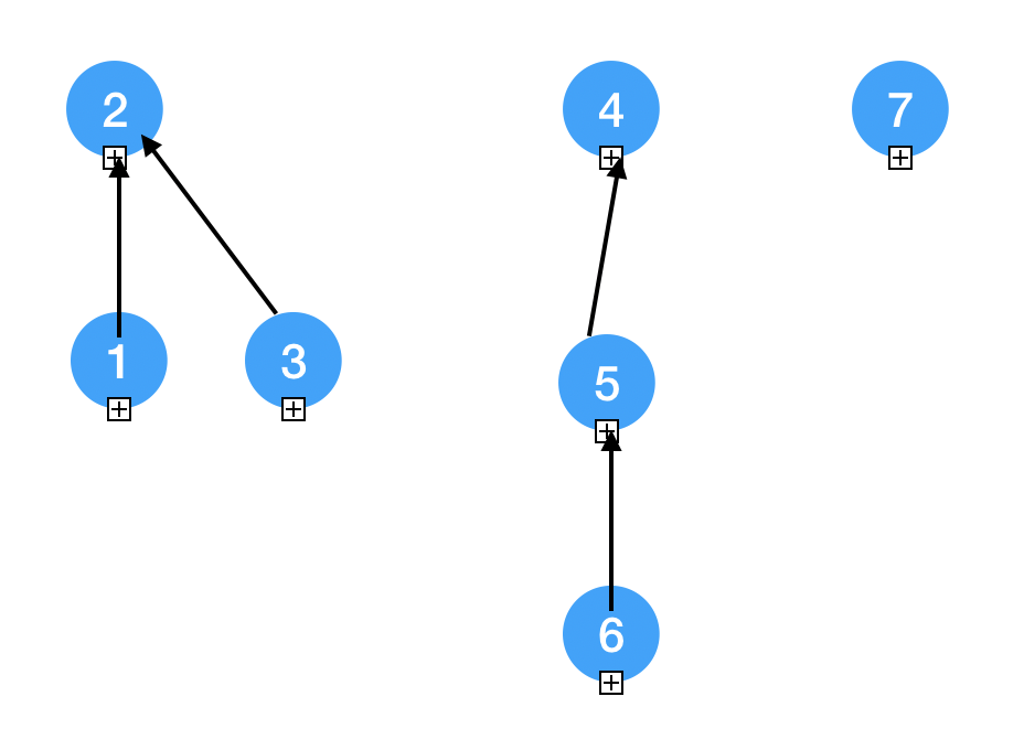
G = [[1, 3], [2, 5], [2, 6], [4, 2], [4, 3], [3, 6]]

After DFS, we have
         1  2  3  4  5  6
timer = [4, 3, 1, 2, 6, 5]

After reverse, 
we have timer = [5, 6, 2, 1, 3, 4]
which is a valid Topological sort.

Step

Use DFS_ALL() find finish time.
Sort vertices by finish time in decreasing order.
Doesn’t work for cyclic graph. Will stuck in the recursion forever.

Pseudocode

// We mark each node in the order we visit them
// if we sort the vertices by decreasing order of finishing time, then I have a valid topological sort
DFS_ALL(G) {
    visited[1...n];
    finish[1...n];
    timer = 1;
    for (u = 1 ... n) {
        if (visited[u] == false) {
            DFS(G, u, visited, finish, timer);
        }
    }

}

DFS(G, u, visited, finish, timer) {
    visited[u] = true;
    for (v in G.neighbor(u)) {
        if (visited[v] == false) {
            DFS(G, v, visited, finish, timer);
        }
    }
    finish[u] = timer;
    timer += 1;
}

// updated version using array as finish time recorder
DFS(G, u, visited, finish) {
    visited[u] = true;
    for (v in G.neighbor(u)) {
        if (visited[v] == false) {
            DFS(G, v, visited, finish);
        }
    }
    finish.append(u);
}

Non DFS Solution

Idea

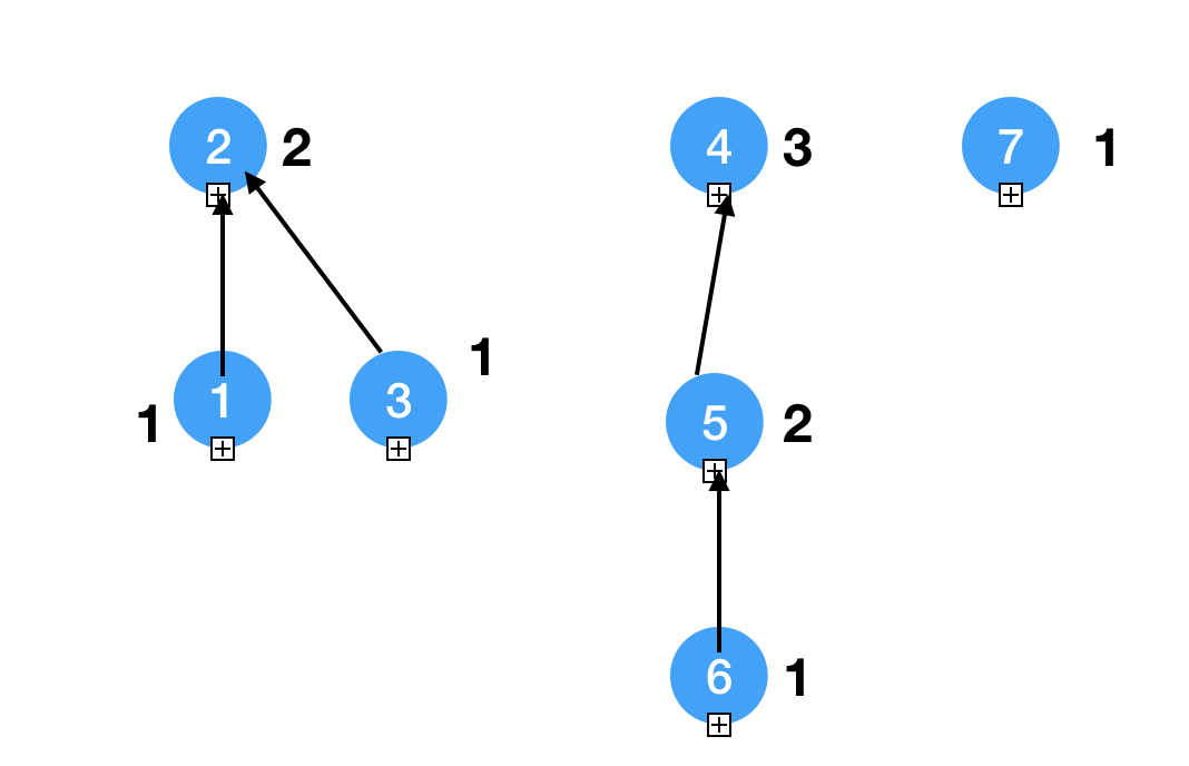
Record the indegree of the vertices and keep searching and updating the indegree map.

The running time is O(m+n)

Pseudocode

TopoSort(G) {
    for (u = 1 ... n) {
        for (v in G[u]){
            in[v]++;
        }
    }
    for (u = 1... n) {
        if (in[u] == 0) q.enqueue(u);
    }
    while (!q.isEmpty()) {
        u = q.dequeue();
        for (v in G[u]) {
            in[v]--;
            if (in[v] == 0) {
                q.enqueue(v);
            }
        }
    }
}

Boggle

Description

Given a 4X4 board

HEAT
ELOI
UYXB
PPAS

Goal: 
- find all words 
- can start at any position
- cannot reuse same pos in the word, but we can reuse them in different words

PseudoCode

// 4^16 Time Complexity. Terrible.
Boggle(B[]) {
    for (int i = 1 ... 4) {
        for (int j = 1 ... 4) {
            DFS(B[], visited[], i, j, "", solution);
        }
    }
    return solution;
}

DFS(B[], visited[], i, j, String cur, solution) {
    visited[i, j] = true;
    potential_word = cur + B[i, j];
    if (dict.contains(potential_word)) {
        solution.add(potential_word);
    }
    if (i > 1 && !visited[i-1, j]) {
        DFS(B[], visited, i-1, j, potential_word, solution);
    }
    if (i < 4 && !visited[i+1, j]) {
        DFS(B[], visited, i+1, j, potential_word, solution);
    }
    if (j > 1 && !visited[i, j-1]) {
        DFS();
    }
    if (j < 4 && !visited[i, j-1]) {
        DFS();
    }
    visited[i, j] = false;
}

def getWords(root):
    temp = root
    import collections
    q = collections.deque()
    q.append(temp)
    res = []
    while q:
        cur = q.popleft()
        if cur.isWord:
            res.append(cur)
        for i in range(26):
            if cur.children[i]:
                q.append(cur.children[i])
    return res

class Trie:
    def __init__(self):
        self.children = [None for _ in range(26)]
        self.word = ""
        self.isWord = False

def boggle(board, dic):
    # Build Trie
    root = Trie()
    for word in dic:
        buildTrie(root, word)
    m, n = len(board), len(board[0])
    res = []
    # DFS
    for i in range(m):
        for j in range(n):
            dfs(i, j, board, root, res, set())
    return res

def buildTrie(root, word):
    temp = root
    # Add all letters to the Trie as nodes
    for letter in word:
        ind = ord(letter) - ord("a")
        if not temp.children[ind]:
            temp.children[ind] = Trie()
        # Update the child and temp
        temp.children[ind].word = temp.word + letter
        temp = temp.children[ind]
    # Last letter node is a valid word
    temp.isWord = True
    
def dfs(i, j, board, root, res, visited):
    # Check if cur Trie Node exists and has been visited or not
    ind = ord(board[i][j]) - ord("a")
    if not root.children[ind] or (i, j) in visited:
        return
    # update cur Trie Node
    root = root.children[ind]
    # Memoization
    visited.add((i, j))
    # Check if we find a result
    if root.isWord:
        res.append(root.word)
    # DFS
    m, n = len(board), len(board[0])
    for dx, dy in [[0, 1], [0, -1], [1, 0], [-1, 0]]:
        tempX, tempY = i + dx, j + dy
        if 0 <= tempX < m and 0 <= tempY < n:
            dfs(tempX, tempY, board, root, res, visited)
    # Backtrack
    visited.remove((i, j))


board = [
    ["a", "a", "c", "d"],
    ["e", "l", "g", "h"],
    ["i", "j", "k", "l"],
    ["m", "l", "a", "a"],
]
dic = ["abc", "aal", "gkjlaaeimlaa", "lmijlgcaae"]
print(boggle(board, dic))

SCC

Description

Every node in this group have access to any other nodes.

d	c
Strongly connected components	u->v and v->u
Weakly connected components	u->v or v->u

Example

G = [[1, 3], [3, 2], [2, 1], [2, 4], [4, 5], [5, 4], [4, 6], [6, 7], [7, 8], [6, 8], [7, 9], [8, 9], [9, 6]]

1. sort by finish time(topological sort)

1 2 3 4 5 6 7 8 9
9 7 8 6 1 5 4 3 2


2. reverse edge direction and do the topo_sort
G = [[3, 1], [2, 3], [1, 2], [4, 2], [5, 4], [4, 5], [6, 4], [7, 6], [8, 7], [8, 6], [9, 7], [9, 8], [6, 9]]


Sort the sequence by decreasing order, and start BFS to this sequence.
9 7 8 6 1 5 4 3 2

Actually, we can start at any node we want when doing the topological sort.
We start from 1, and get 1, 3, 2
then start from 4, get 4, 5
then 6, get 6, 9, 8, 7
that's the scc groups we want

Steps

Do topological sort on G(DFS)
BFS in GT using sequence produced by step 1

SSSP

Description

SSSP = single source shortest path
given Graph, we need to find every shortest path from the source S to other nodes.

Pseudocode

negative weighted edges	DAG	not DAG	Time
N	SP on DAG, O(m+n)	Dijkstra’s algo	Omlogn(sparse) or O n^2(dense)
Y	Same as above	Bellmen Ford	O(mn)

Class 12 07/29/2019

Single Source Shortest Path

Description

Given G and s, return a dist[u] which stores the shortest disatnce from s to u.

Shortest Path on DAG

Description

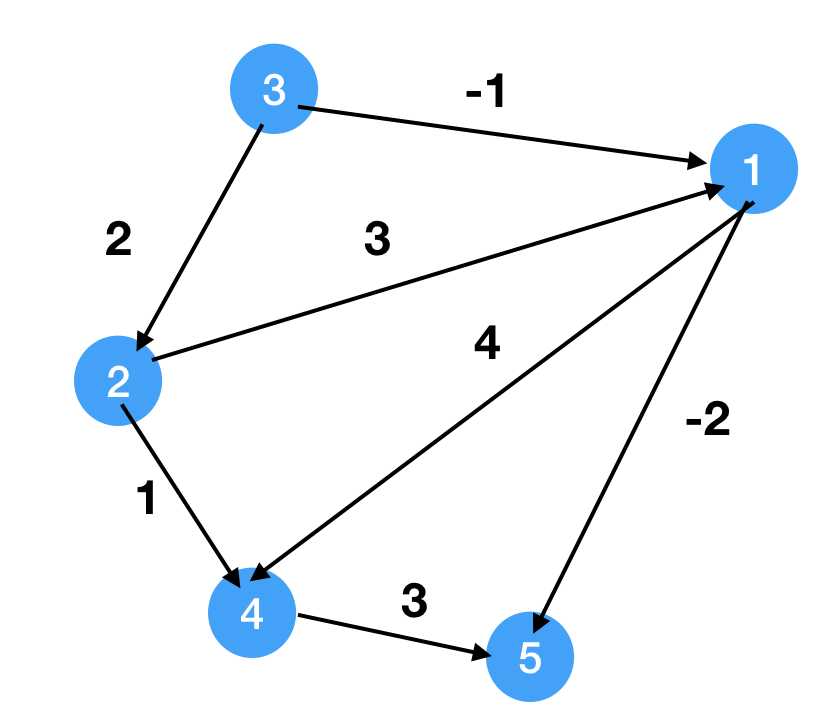
input: G(V, E), S
step:
0. dist[S] = 0, dist[others] = inf
1. topological sort
2. relax the edge(u, v)

Time Complexity O(m+n)

PseudoCode

// helper function, check if v is the shortest path given u.
relax(u, v) {
    // Cuv = Cost from u to v
    if (dist[u] + Cuv < dist[v]) {
        dist[v] = dist[u] + Cuv
    }
}
getShortest(G) {
    topological_sort = topo_sort(G);
    dist = [inf ... 0...inf]; // Set all to inf except s
    for (u in topological_sort) {
        for (v in G.neighbor(u)) {
            relax(u, v);
        }
    }
    return dist;
}

Example

topo = [3, 2, 1, 4, 5]
dist = [inf, inf, 0, inf, inf]
        -1,   2 , 0, inf, inf           3
        -1,   2,  0,  3 , inf           2
        -1,   2,  0,  3 , -3            1
        -1,   2,  0,  3 , -3            4
        -1,   2,  0,  3 , -3            5
Q: Why is Topological sort working?
dist[u] = min(dist[x] + Cxu, dist[y] + Cyu), Assume x and y is before u. We need to finish all prerequisites before we try to update u, which is sorted by topological sort.

Dijkstra’s algorithm

Description

Get the dist[], N is set of the vertices we vistited.
n is the total number of vertices.
while (|N| != n) {
    1. pick vertex u in V but not in N with the smallest dist[] value
    2. N.add(u)
    3. for all neighbors of u, relax them.
}

Example

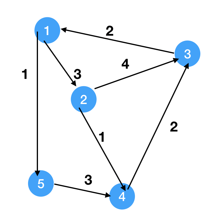
S = 2
N = {}
dist = [inf, 0, inf, inf, inf]

1. u = 2, N = {2}, relax(2, 1), relax(2, 3), dist = [inf, 0, 4, 1, inf]
2. u = 4, N = {2, 4}, relax(4, 3), dist = [inf, 0, 3, 1, inf]
3. u = 3, N = {2, 4, 3}, relax(3, 1), dist = [5, 0, 3, 1, inf]
4. u = 1, N = {2, 4, 3, 1}, relax(1, 2), relax(1, 5), dist = [5, 0, 3, 1, 6]
4. u = 5, N = {2, 4, 3, 1, 5}, relax(5, 4), dist = [5, 0, 3, 1, 6]

Analysis

1. pick a smallest distance node, O(n)
2. Add the node to my set, set[node] = true, O(1)
3. relax u's neighbors, O(du), Dout < n.
4. Overall is n * n = n^2

Using min heap
1. pick u, O(1)
2. delete u, O(logn) and add to the set, O(1)
3. relax it's neieghbors, O(Du * logn).
## Here we just need to bubble up the changed node 
4. Overall is O(mlogn) = d1logn + d2logn + ... + dnlogn = mlogn

Bellman Ford

Description

Relax all edges n-1 times.

Example

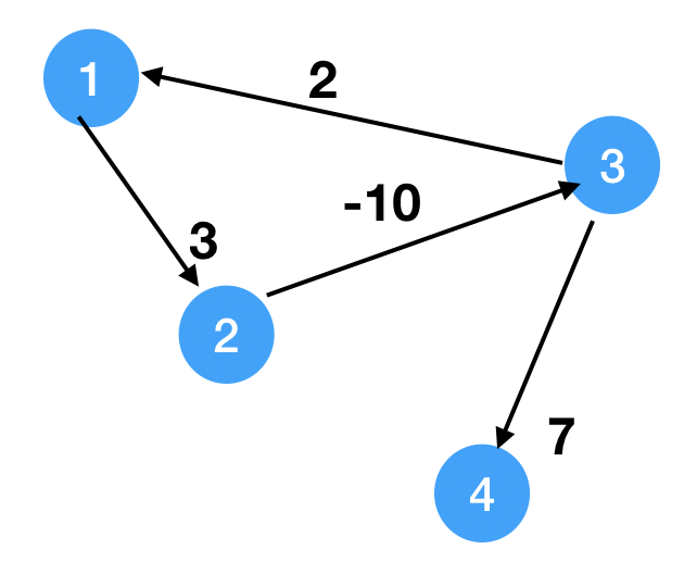
S = 1
dist = [0, inf, inf, inf]
i = 1, we get 2, 3, 4, 1, dist = [0, 3, inf, inf]
i = 2, we get 2, 3, 4, 1, dist = [0, 3, -7, 0]
i = 3, dist = [0, 3, -7, 0]

Since we can at least update one true shortest distance at each loop, then we need at most n-1 times to update all true shorteset distances. After that, the dist array shouldn't change. If it changes, it means there's a cycle with negative weights.

PseudoCOde

for (i = 1... n-1) {// we do the algo n-1 times
    for (u = 1...n) {
        for (V in G.neighbors(u)) {
            relax(u, v);
        }
    }
}

Class 13 08/05/2019

Review

Shortest path on DAG, O(m+n)
Dijkstra’s Algorithm, O(mlogn) for pq, O(n^2) for matrix
Bellman Ford Algorithm, O(mn)
How do we track the actual paths? we need to modify the relax function.

relax(u, v) {
    if (dist[u] + cur < dist[v]) {
        dist[v] = u;
        parent[v] = u;
    }
}

All Pair Shortest Path

Description

Goal: Build dist[u, v] = shortest distance from u to v

negative weighted edges	DAG	not DAG	Time
N	O(mn) = On^2 ~ On^3	Dijkstra’s algo	Onmlogn = O n2logn ~ n3logn or O n^3
Y	m = n(n-1) at most	Bellman Ford	O(mn^2) = On3 ~On4

To improve the time complexity of Bellman Ford Algorithm interms of number of vertices, we can use Floyd-Warshall Algorithm.

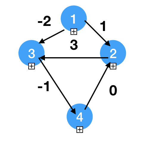
Floyd - rWarshall Algorithm

Description

We define f_k(u, v) = shortest distance from u to v with only vertices{1, 2, … k} on shortest path

Example:
f_1(u, v) = 20
f_2(u, v) = 7

f_k(u, v) = cur, if (u, v) in E
            inf, otherwise

base case:
f_0(u, v) = inf, if such edge doesn't exist
            weight(u, v), otherwise
f(u, u) = 0

Recurrence:
f_1(u, v) = min(f_0(u, v), f_0(u, 1) + f_0(1, v))
f_k+1(u, v) = min(f_k(u, v), f_k(u, k+1) + f_k(k+1, v))

f_n(u, v) = true shortest distance {1, 2, 3, ..., n}

PseudoCode

FW(G) {
    dist[,] = adj matrix
    for (k = 1, 2, ..., n) {
        for ( u = 1 ... n) {
            for (v = 1 ... n) {
                dist[u, v] = min(dist[u, v], dist[u, k] + dist[k, v]);
            }
        
    }
}

Example

Adj matrix

0, 1, -2, inf
inf, 0, 3, inf
inf, inf, 0, -1
inf, 0, inf, 0

k = 1
dist[1, 1] = inf
dist[1, 2] = min(1, dist[1, 1] + dist[1, 2]) = 1
dist[1, 3] = min(-2, dist[1, 1] + dist[1, 3]) = -2
dist[1, 4] = min(inf, dist[1, 1] + dist[1, 4]) = inf

dist[2, 3] = min(dist[2, 3], dist[2, 1] + dist[1, 3]) = min(3, inf + (-2)) = 3

The first iteration basically doesn't change
k = 2
dist[1, 1] = min(inf, dist[1, 2] + dist[2, 1]) = inf
dist[1, 3] = min(-2, dist[1, 2] + dist[2, 3]) = min(1, 4) = 1

dist[4, 3] = min(inf, dist[4, 2] + dist[2, 3]) = 3


0, 1, -2, inf
inf, 0, 3, inf
inf, inf, 0, -1
inf, 0, 3, 0

k = 3
dist[1, 4] = min(inf, -2 + -1) = -3
dist[2, 1] = min(inf, 0 + inf) = inf
dist[2, 3] = min(3, 3 + 0) = 3
dist[2, 4] = min(inf, 3 + -1) = 2

...

Negative weighted cycle is not applicable!

Minimum Spanning Tree

Description

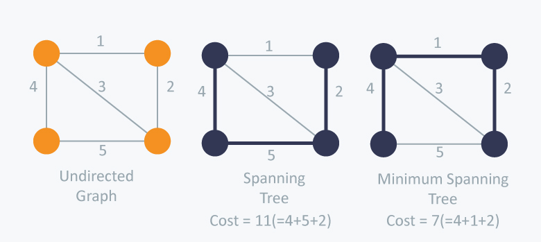
1
2
3

Input: Connected undirected graph
we want to find a weighted undicted graph that has the smallest cost.
We have Prim's Algorithm and Kruskal's Algorithm to solve this.

Prim’s Algorithm

Description

N = {}
dist[u] = distance from set N to vertex U
N is a set of vertices, we pick the shortest distacne from amongst all possible edges from U to this set.

Example, 
N = {}, dist = inf, inf, inf, inf
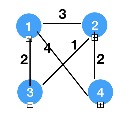
1. N = {3}, dist = 2(3, 1), 1(3, 2), 0, inf
2. N = {3, 2}, dist = 2(3, 1), _, _, 2(4, 2)
3. N = {3, 2, 4}, dist = 2(3, 1), _, _, _
4. N = {3, 2, 4, 1}, dist = _, _, _, _

Final dist = [2, 1, 0, 2]

Final Spanning Tree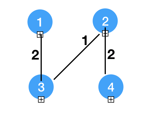

PseudoCode

Prims(G) {
    N = {}, T = {};
    while (N != V) {
        1. pick vertex u in (V/N) with the smallest distance value
        2. N = N U {u}, T = {(u, parent(u))} U T
        3. for (v in G.neighbor(u)) {
            if (Cost(u, v) < dist[v]) {
                dist[v] = Cost(u, v), T[v] = u;
            }
        }
    }
}

Example

N = {3}
dist = [2, 1, inf, inf]
parent = [3, 3, -1, -1]

N = {3, 2}
dist = [2, 1, inf, 2]
parent = [3, 3, -1, 2]

N = {3, 2, 4}
dist = [2, 1, inf, 2]
parent = [3, 3, -1, 2]

N = {3, 2, 4, 1}
dist = [2, 1, inf, 2]
parent = [3, 3, -1, 2]

Our Tree is (1, 3), (2, 3), (4, 2)

Actually here we don't need T here, and we can use a priority Queue to pick the smallest distance not in N.

Kruskal’s Algorithm

Description

- Sort edges by their weights
- T = {}
for (e in sorted order) {
    if (T U {e} has no cycle) {
        T = T U {e}
    }
}
To detect cycle, we can either use disjoint sets.

Disjoint Sets

1 2	- We have n items {1, 2, ..., n} - group them into disjoint sets {1, 2}, {4, 5, 6}

// mlogn time 
for (e = (u, v) in sorted order) {
    if (Find(u) != Find(v)) {
        T = T U {(u, v)}; // union
        Union(u, v);
    }
}

Union Find

Logical View

1 2	1 2 3 4 5 6 7 2 2 2 4 4 5 7

PseudoCode

Find(u) {
    if (parent[u] == u) {
        return u;
    }
    return Find(parent[u]);
}

Union(u, v) {
    parent[u] = v;
}

Union By Rank

/**
1 2 3 4 5 6 7
1 2 1 3 2 1 1
Find O logn Union O 1

num of item of a root node >= 2 ^(rank - 1)
proof:
if rank = 1, then 1 >= 2^1 - 1
assume rank = k, node >= 2^(k-1)
when rank = k+1, assume target = 2^k, we have node + node >= 2^(k-1) * 2 = 2^k >= target. Thus the time complexity is O logn
**/
// we need to find first
u = find(u);
v = find(v);
if (rank[u] < rank[v]) {
    parent[u] = v;
} else if (rank[u] > rank[v]) {
    parent[v] = u;
} else {
    parent[u] = v;
    rank[v]++;
}

Path Compression

We dont want a long chain here, we want less levels of nodes. So we modify the parent of the node to be the root each time we find.

Assume for a sequence of m U&F operations.
overall running time , O(mlog*n).

eg.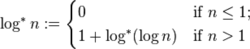

log 2 = 1
log 4 = 2
log 16 = 3
log 65536 = 4
log* 2^65536 = 5

Find(u) {
    if (parent[u] == u) {
        return u;
    }
    parent[u] = Find(parent[u]);
    return parent[u];
}